Financial models with long-tailed distributions and volatility clustering
Financial models with long-tailed distributions and volatility clustering have been introduced to overcome problems with the realism of classical financial models. These classical models of financial time series typically assume homoskedasticity and normality cannot explain stylized phenomena such as skewness, heavy tails, and volatility clustering of the empirical asset returns in finance. In 1963, Benoit Mandelbrot first used the stable (or  -stable) distribution to model the empirical distributions which have the skewness and heavy-tail property. Since -stable distributions have infinite
  -th moments for all
  , the tempered stable processes have been proposed for overcoming this limitation of the stable distribution.
On the other hand, GARCH models have been developed to explain the volatility clustering. In the GARCH model, the innovation (or residual) distributions are assumed to be a standard normal distribution, despite the fact that this assumption is often rejected empirically. For this reason, GARCH models with non-normal innovation distribution have been developed.
Many financial models with stable and tempered stable distributions together with volatility clustering have been developed and applied to risk management, option pricing, and portfolio selection.
Contents |
Infinitely divisible distributions
A random variable  is called infinitely divisible if, for each
  , there are independent and identically-distributed random variables
such that
where  denotes equality in distribution.
A Borel measure  on
on  is called a Levy measure if
  and
and
If is infinitely divisible, then the characteristic function ![\phi_Y(u)=E[e^{iuY}]](/2012-wikipedia_en_all_nopic_01_2012/I/7ce24c0cd2b54b5a917f9703f08ee96d.png) is given by
is given by

where  ,
,  and is a Levy measure. Here the triple
  is called a Levy triplet of . This triplet is unique. Conversely, for any choice satisfying the conditions above, there exists an infinitely divisible random variable whose characteristic function is given as
  .
.
α-Stable distributions
An real-valued random variable  is said to have an -stable distribution if for any
  , there are a positive number
  and a real number
  such that
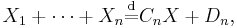
where  are independent and have the same distribution as that of . All stable random variables are infinitely divisible. It is known that
  for some
  . A stable random variable with index is called an -stable random variable.
Let be an -stable random variable. Then the characteristic function  of is given by
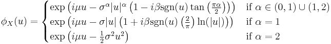
for some  ,
,  and
and ![\beta\in[-1,1]](/2012-wikipedia_en_all_nopic_01_2012/I/d04404bfa3e977d2d425336e7c4257bd.png) .
.
Tempered stable distributions
An infinitely divisible distribution is called a classical tempered stable (CTS) distribution with parameter  , if its Levy triplet is given by
  , and
, and
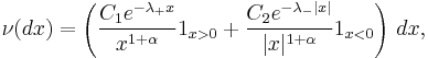
where  and
and  .
.
This distribution was first introduced by under the name of Truncated Levy Flights[1] and has been called the tempered stable or the KoBoL distribution.[2] In particular, if  , then this distribution is called the CGMY distribution which has been used for financial modeling.[3]
The characteristic function  for a tempered stable distribution is given by

for some . Moreover, can be extended to the region  .
.
Rosiński [6] generalized the CTS distribution under the name of the tempered stable distribution. The KR distribution, which is a subclass of the Rosiński's generalized tempered stable distributions, is used in finance.[4]
An infinitely divisible distribution is called a modified tempered stable (MTS) distribution with parameter  , if its Levy triplet is given by , and
where  and
and
Here  is the modified Bessel function of the second kind. The MTS distribution is not included in the class of Rosiński's generalized tempered stable distributions.[5]
Volatility clustering with stable and tempered stable innovation
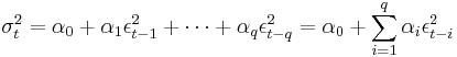
In order to describe the volatility clustering effect of the return process of an asset, the GARCH model can be used. In the GARCH model, innovation ( ) is assumed that
  , where
  and where the series
  are modeled by
and where  and
and  .
.
However, the assumption of is often rejected empirically. For that reason, new GARCH models with stable or tempered stable distributed innovation have been developed. GARCH models with -stable innovations have been introduced.[6][7][8] Subsequently, GARCH Models with tempered stable innovations have been developed.[5][9]
Notes
- ^ Koponen, I. (1995) "Analytic approach to the problem of convergence of truncated Levy flights towards the Gaussian stochastic process", Physical Review E, 52, 1197–1199.
- ^ S. I. Boyarchenko, S. Z. Levendorskiǐ (2000) "Option pricing for truncated Levy processes", International Journal of Theoretical and Applied Finance, 3 (3), 549–552
- ^ P. Carr, H. Geman, D. Madan, M. Yor (2002) "The Fine Structure of Asset Returns: An Empirical Investigation", Journal of Business, 75 (2), 305–332.
- ^ Kim, Y.S.; Rachev, Svetlozar. T.;, Bianchi, M.L.; Fabozzi, F.J. (2007) "A New Tempered Stable Distribution and Its Application to Finance". In: Georg Bol, Svetlozar T. Rachev, and Reinold Wuerth (Eds.), Risk Assessment: Decisions in Banking and Finance, Physika Verlag, Springer
- ^ a b Kim, Y.S., Chung, D. M. , Rachev, Svetlozar. T.; M. L. Bianchi, The modified tempered stable distribution, GARCH models and option pricing, Probability and Mathematical Statistics, to appear
- ^ C. Menn, Svetlozar. T. Rachev (2005) "A GARCH Option Pricing Model with -stable Innovations", European Journal of Operational Research, 163, 201–209
- ^ C. Menn, Svetlozar. T. Rachev (2005) "Smoothly Truncated Stable Distributions, GARCH-Models, and Option Pricing", Technical report. Statistics and Mathematical Finance School of Economics and Business Engineering, University of Karlsruh
- ^ Svetlozar. T. Rachev, C. Menn, Frank J. Fabozzi (2005) Fat-Tailed and Skewed Asset Return Distributions: Implications for Risk Management, Portfolio selection, and Option Pricing, Wiley
- ^ Kim, Y.S.; Rachev, Svetlozar. T.; Michele L. Bianchi, Fabozzi, F.J. (2008) "Financial market models with Levy processes and time-varying volatility", Journal of Banking & Finance, 32 (7), 1363–1378 doi:10.1016/j.jbankfin.2007.11.004
References
- B. B. Mandelbrot (1963) "New Methods in Statistical Economics", Journal of Political Economy, 71, 421-440
- Svetlozar. T. Rachev, S. Mitnik (2000) Stable Paretian Models in Finance, Wiley
- G. Samorodnitsky and M. S. Taqqu, Stable Non-Gaussian Random Processes, Chapman & Hall/CRC.
- S. I. Boyarchenko, S. Z. Levendorskiǐ (2000) "Option pricing for truncated Levy processes", International Journal of Theoretical and Applied Finance, 3 (3), 549–552.
- J. Rosiński (2007) "Tempering Stable Processes", Stochastic Processes and their Applications, 117 (6), 677–707.